Contents

Divide and Conquer

In computer science, when faced with certain types of problems, we can turn to a method called divide and conquer. This method will not work or be appropriate for every problem we encounter, but for a certain class of problems, it is extremely helpful. As the name suggests, divide and conquer is the process of breaking a problem into similar subparts, that can be broken into similar subparts, that can be broken into similar subparts...etc. etc. etc., until there's nothing left to consider. When functions are used to compute the subparts, we call this nesting recursion (think about pointing a video camera at the TV that's displaying the feed—the TV is showing the TV is showing the TV is showing the TV .... only with our recursion, we're going to stop at some point). In recursion, we the function we use to operate on a subpart considers the subpart it's given and will either decide it's small enough to return an answer (called the base case), or it breaks the subpart into one or more smaller chunks and then invokes itself with the smaller chunks. At some point, the base case will be reached and the function will return, which will cause the previous function to return, which will cause the next previous function to return, etc.

As an initial example, let's consider the mathematical operation factorial. Written as n!, where n is any number, the factorial function will produce the product: n×(n-1)×(n-2)×....×1. It problem seems clear how you could compute this with a loop. But just to get the concept of recursion across, let's consider another way of looking at n!. It's also equal to: n×(n-1)!. Using pseudo code, lets see how we can take this insight and create a recursive solution to solving it.

Define function factorial
Input:  a number n
Output: the factorial of n

    // Base case: 
    if n equals 1, return 1 
    // Recursive case:
    otherwise, return (n × factorial(n-1))

So our base case simply checks if we've reached the end of the sequence (1) and if so, returns 1. Our recursive case strips off n—the current number in the sequence—and returns the product of it with the factorial of the next number in the sequence (n-1).

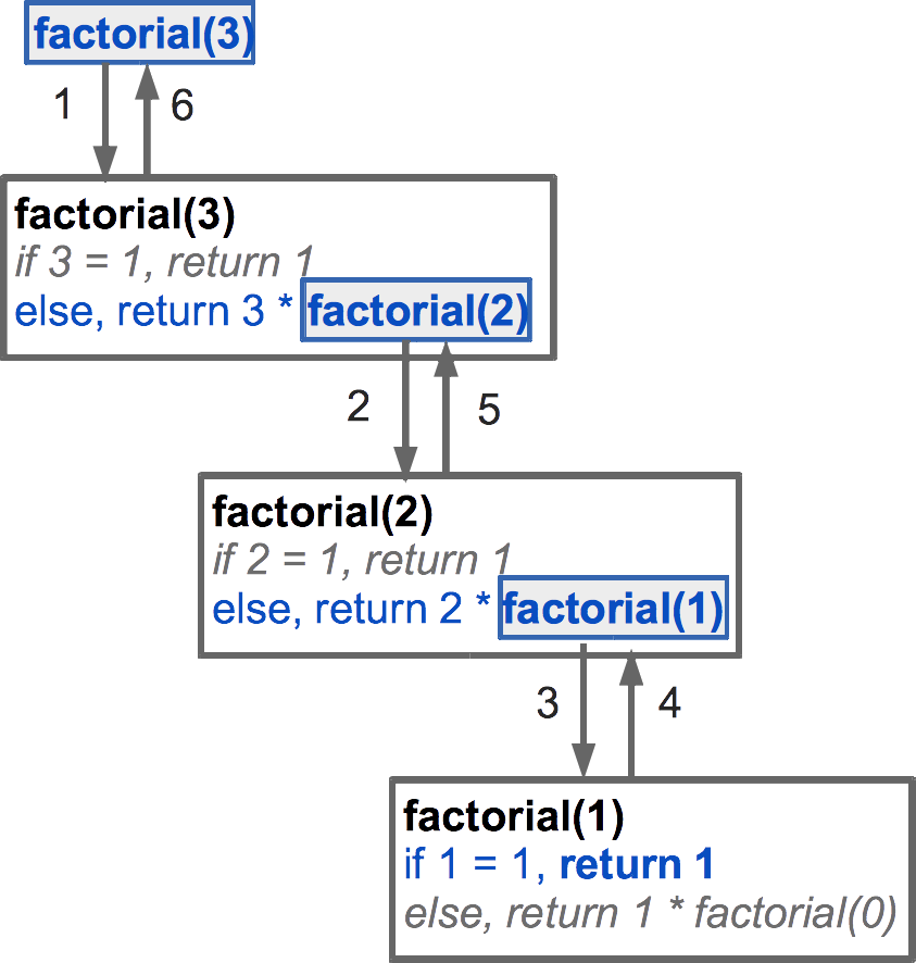
Let's consider what happens if we call factorial(3). In this first invocation, we check the base case. Since 3 ≠ 1, we continue to the recursive case. Here's we want to return the product of 3 and factorial(2). Before the multiplication or return can occur, we must first invoke factorial and wait it to return. So our current invocation is just hanging out until it hears back from factorial(2). I this second invocation, factorial(2), we check the base case, which isn't met as 2 ≠ 1. So we go to the recursive case and return the product of 2 and factorial(1). As before, we can't perform the multiplication or the return until factorial(1) has returned, so now our second invocation is also just sitting around waiting. In the third invocation, factorial(1), we check the base case, and this time, the criteria are met: 1 = 1 (woohoo!). So that means we return 1. Good. This causes control to go back to the second invocation, which can now multiple 2 × 1 and return 2. This return gives control back to our first invocation, where we need to multiple 3 × 2 and return 6. That returns control to wherever we originally invoked factorial(3), and we have our answer: 6. \ref shows a visualization of the invocations.

Direct and Indirect recursion

If a recursive solution involves a function that directly calls itself, just as in our factorial example above, we call that direct recursion. It is sometimes helpful to have a set of two or three functions that work together to complete a recursive solution. Lets suppose we have two functions, f1 and f2. Our solution may involve f1 invoking f2, which in turn invokes f1, and so on. Since f1 does not call itself, but does call f2 which then invoked f1, we can say that f1 is indirectly recursive. In this particular situation, we can say the same for f2. We will see some practical examples of indirect recursion later in the semester, but for now, consider the following recursive approach to printing an alternating sequence of tildes (~) and plus signs of total length n in pseudo code:

Define the function printTilde
Input:  a length n
Output: nothing

    // Base case:
    if n equals 0, return nothing
    // Recursive case:
    otherwise:
        print "~"
        invoke printPlus(n-1)


Define the function printPlus
Input: a length n
Output: nothing

    // Base case:
    if n equals 0, return nothing
    // Recursive case:
    otherwise:
        print "+"
        invoke printTilde(n-1)

Single and multiple recursion

The examples we've seen so far have used single recursion (or linear recursion), wherein we make at most one recursive call within any case of our function. Some recursive solutions require multiple recursive calls, and we call this multiple recursion. A classic example of this is the recursive solution to computing the n^th number in the Fibonacci sequence. The Fibonacci sequence starts with 1, 1, and then every number after that is the sum of the previous two numbers in the sequence. For example, the third number in the sequence is Fibonacci(3) = Fibonacci(2) + Fibonacci(1) = 1 + 1 = 2. See how to the right of the equal sign we have two invocations of the Fibonacci function? That makes this a case of multiple recursion.

Tail recursion

If a return value of a recursive function includes only a recursive call (e.g., with no other computations as part of the statement), then it is called tail recursive. For instance, \ref is tail recursive since the return statement includes only a recursive call to printPlus or printTilde. Tail recursion is the easiest form of recursion to translate into an iterative solution. Compilers for many programming languages will automatically convert single, tail recursive functions into loops when generating machine code, because they are relatively easy to detect and the iterative solution is often more efficient than the recursive one (more on that in Section \ref).

Implementing Recursion in C++

We do not need any special syntax to implement recursion in C++, just regular old functions. Here's what our factorial example looks like as a fully working C++ program:

The call stack

In C++, as in many languages, function invocations involve allocating memory for a new instance of the function, including all its variables, and then keeping that memory around until the function has returned. In recursion, a function cannot return until all the functions "below" it have returned, which can only happen when the base cases have been met. \ref demonstrates this for the factorial example. That example, however, only has three concurrent instances of the function. Consider problems where there are thousands or even millions of subproblems—that can be a lot of information on the call stack.

Recursion is not always the preferred solution

Due to the cost of function invocations and stack storage, recursion is not always the preferred method. In fact, if you take a working solution that uses loops (which we call an iterative approach) and convert it into a recursive solution, you may find that your C++ will crash due to a filled call stack.

Given that caveat, you may be wondering why we even bother with recursion. For the problems where recursive solutions are a good fit, the iterative solutions are complex, ugly, and difficult to comprehend: the recursive solutions are typically concise, elegant, and simple to understand. So you must weigh this with the potential downfalls, which are mostly due to the call stack.

(Back to top)