Contents

Sorting lists

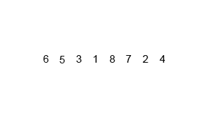
We saw that sorting lists of data makes searching them more efficient. In this topic, we'll go over some of the ways to sort arbitrary data. Just as an example, we'll use this short list of numbers when explained several of the algorithms:

5

10

3

20

8

(Back to top)

Bubble sort

Bubble sort is one of the simplest sorts. It's also among the most expensive. For a list of length n, it makes n passes. On each pass, it walks the list from left (index 0) to right, ending at the second-to-last item (index n-2). For each item, it compare the item to its neighbor to the right. So the item at index 0 is compared to the item at index 1. If the one on the left is greater than the one to the right, they are swapped. Then it increments the current index and does the same thing. After making n passes, the list will be sorted because all of the "larger" items will "bubble" to the right. Here's an example using our unsorted array from \ref:

5

10

3

20

8

5

10

3

20

8

5

3

10

20

8

5

3

10

20

8

5

3

10

8

20

Here's what the array will look like after each of the next four passes:

3

5

8

10

20

Even though we were actually done sorting after the second pass, we would have needed the other three passes if our data had been sorted in the exact opposite order (the worst case scenario). Here's a look at what happens after each pass if we start with the list backwards (the green boxes are elements that are in their correct sorted position):

20

10

8

5

3

10

8

5

3

20

8

5

3

10

20

5

3

8

10

20

3

5

8

10

20

3

5

8

10

20

Even though it doesn't look like it, we need this last pass to ensure that 3 is in the correct spot. So, in the worst case, we make n passes, each of which makes up to n comparisons. Therefore, our complexity is O(n²).

Wikipedia has a nice animated GIF of the process:

A slightly smarter bubble sort

Although it won't help the worst case complexity, we can ensure that our bubble sort will stop early if the list is sorted. What we can do is keep track of how many swaps we have made during the current pass. If we haven't made any, then the list hasn't changed, which will only be true if it is already sorted. So, in our original bubble sort example, we would perform the first and second pass. Because we did make a swap in the second pass, we'd still have to make a third pass, even though the list is sorted. In the third pass, however, we don't perform any swaps, so we don't have to make the fourth or fifth pass. In or example where we started with the list in reverse order, we would still have to do all five passes.

(Back to top)

Insertion sort

Insertion sort is another relatively simplistic algorithm, and indeed has the same worst case complexity as bubble sort: O(n²). With insertion sort, we work our way from the left to the right of the list. Everything to the left of the current position is sorted, everything to the right is unsorted. At each step, we insert the item we are currently looking at where it belongs in the sorted items to the left of that position, and, in the case that we are working with an array, shift everything from the sorted side that is greater than the current item to the right one position to make room for the item. We then move on to the next unsorted item.

Wikipedia has a nice animated GIF of the process:

So why is it O(n²)? Because the worst case, when the list is in reverse sorted order, requires that each item be moved to the very left-most spot, causing n comparisons. Since there are n items, we get a complexity of O(n × n) = O(n²).

(Back to top)

Selection sort

Yet another simple sorting algorithm is selection sort, and like the other simple sorting algorithms, has a worst case complexity of O(n²). Selection sort starts with a pointer at index 0. It then walks down the list and finds the minimum item. This is then swapped with the item at the pointer. The pointer is then advanced and we walk from the pointer to the end of the list searching for the minimum. We keep doing this until the pointer has reached the last index, at which point, the list is sorted. Here's the first two passes of our example:

↓
5	10	3	20	8

↓
5	10	3	20	8

↓
3	10	5	20	8

	↓
3	10	5	20	8

	↓
3	10	5	20	8

	↓
3	5	10	20	8

		↓
3	5	10	20	8

We wind up with O(n²) because we have to perform n passes, and we need to perform as many as n comparisons during each pass to find the minimum item, so n × n comparisons.

(Back to top)

Quick sort

Another sort, called quick sort, is, in the worst case, as poor a choice as both bubble and insertion sort. However, in the typical case, quick sort is O(n log₂ n). Here's how it works. First, you pick a pivot item. This can be done at random (to make it easy, just pick the first item). Next, we make two sublists: one with all the items that are smaller than the pivot item, and another with all the larger items. This is called the partition step. Now we do exactly the same process to each of the sublists (i.e., it's a multiple recursion algorithm). We then glue the sorted sublist of smaller items, the pivot, and the sorted sublist of bigger items. Here's the steps for our array in \ref. The pivot is the orange box.

5

10

3

20

8

	5
3			10	20	8

	5
3			10	20	8

	5
3			10
		8		20

	5
3			10
		8		20

	5
3		8	10	20

3

5

8

10

20

So, when is this O(n log₂ n)? Provided that we pick "good" pivots for each list/sublist (i.e., ones that will evenly split the list), then we should wind up with log₂ n distinct pivots. That's because we need as many pivots as n can be divided by 2. The n coefficient comes from the fact that each of the n items in the list needs to, in the limit, be compared to each of the pivots. So, we get O(n log₂ n). Now, as we said earlier, this is the average case, not the worst case. In the worst case, we get O(n²). Why? Because if we always choose a crappy pivot, i.e., one that is the minimum or maximum for its list/sublist, then we end up with n pivots. That would require a lot of bad luck, but it can happen. So, the worst case is bad, but in practice, this algorithm is usually very...quick.

(Back to top)

Merge sort

Merge sort is another recursive algorithm. However, unlike the previous methods, it runs in O(n log₂ n) in its average and worst case. That's a pretty solid guarantee. So how's it work? Each step of the recursion takes an unsorted list. If the list only have one thing in it, it's returned. Otherwise, divide the list in two and sort each half by making a recursive call. Then, merge the resulting sublists; this requires first looking at (we'll call this "pointing to") the first item of each list. Take the smaller item of the two being pointed to and append that to the merged list; advance the corresponding pointer so it points to the next item in that list. Keep doing this until all items have been taken from both sublists. Return the merged list. That's it!

Here's an animated GIF courtesy of Wikipedia:

So why is this O(n log₂ n). The log₂ n comes from the fact that we divide the list in half each time. We can divide a list of length n in half log₂ n times. For each merge step, we perform n comparisons. Thus, since there are log₂ n merges, we wind up with a total of n log₂ n comparisons.

While merge sort is faster than quick sort, optimized implementations of quick sort are often used in sorting libraries for programming languages. However, merge sort is found in the libraries of many other programming languages. There is one other sort that is sometimes used, which we will not cover, called heap sort. Heap sort is a variation of selection sort, and depends on a data structure called heap, which we will use when we discuss priority queues.

(Back to top)

Other sorts

There are many other specialized sorts, e.g., made especially for integers or strings. In addition, there are many data structures that sort data automatically upon insertion. For instance, Binary Search Trees and heaps. For the curious, take a look at the Wikipedia page on sorting algorithms.

(Back to top)